writing programs with language models
With infinite compute, program synthesis is trivial – iterate through all programs for one that works. In practice, we need to find a working program with as few samples as possible. This post covers how to generate good programs using language modeling.
Let’s start with a short recap of last post.
the problem
The task is make a rectangle that keeps the grass coordinates inside, and mushroom coordinates outside. This task is represented as a specification of input-outputs, spec, given below.

the ground-truth distribution
Given this particular spec, let’s look up its row M[spec,:] in the meaning matrix. For every rectangle (the program), this row contains information on whether it is correct on our spec.
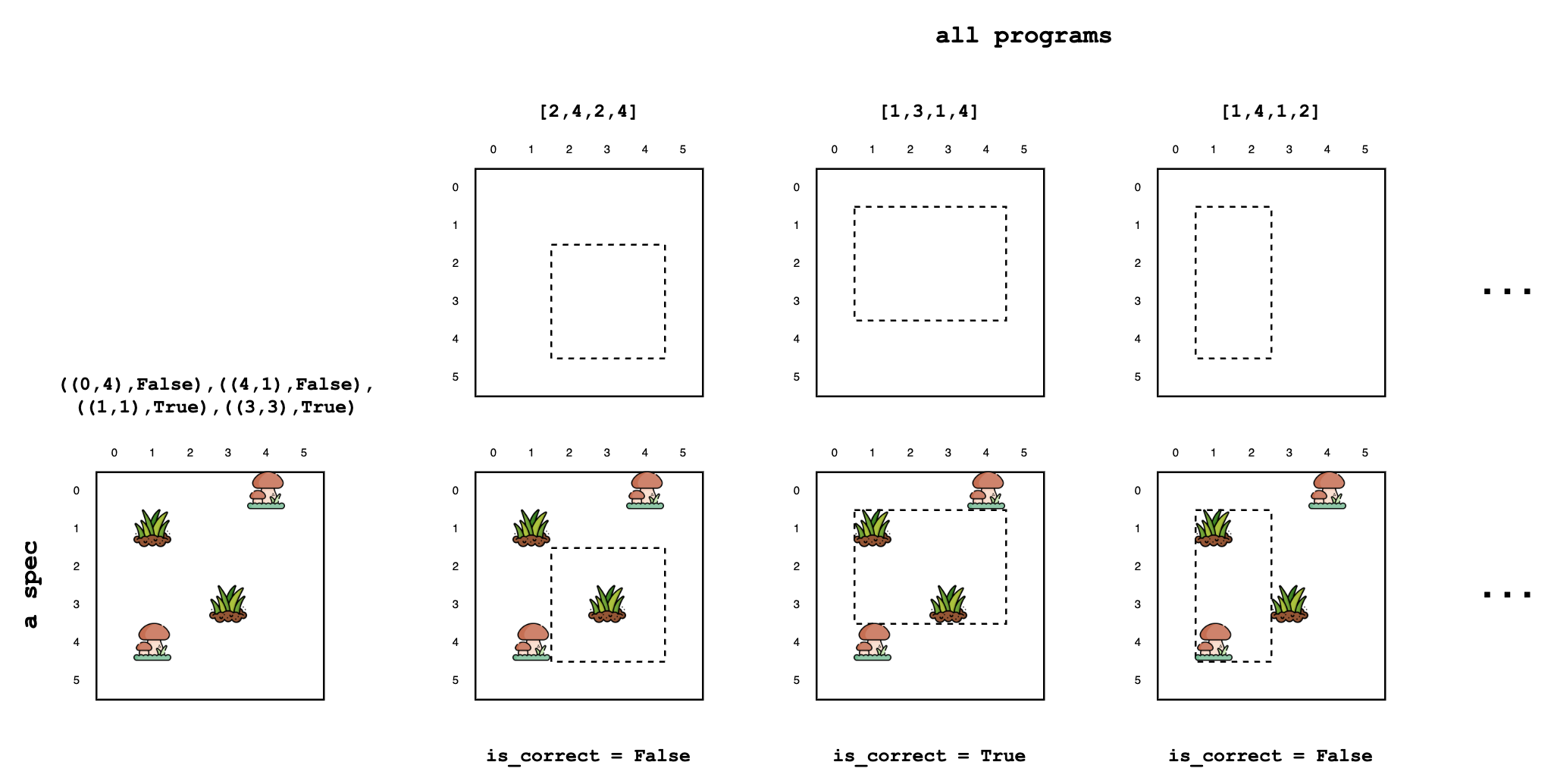
Given spec, the ground-truth distribution for program synthesis can be constructed by first counting1 the number (N) of correct programs, and putting a weight of 1/N on each.
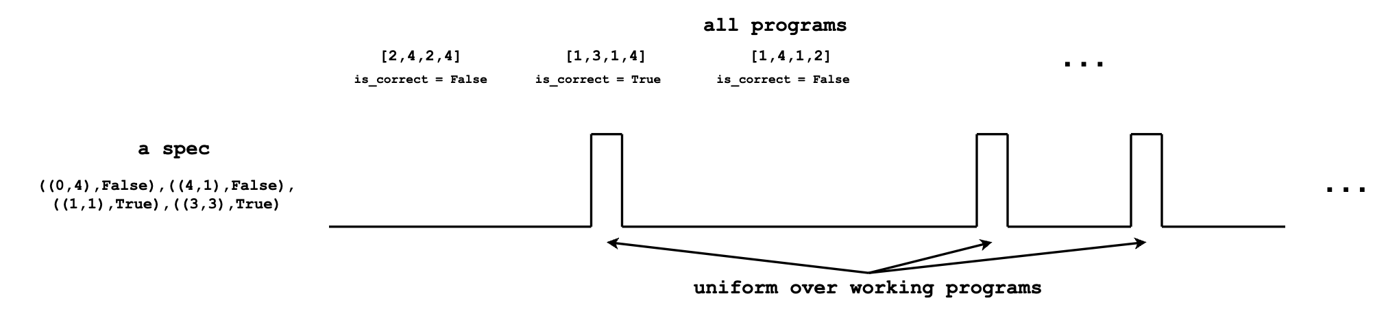

Program synthesis requires us to sample from this ground-truth distribution. Unfortunately, sampling from the ground-truth distribution is hard. While we can easily check if a program is correct given the spec, coming up with correct programs is difficult.
program synthesis as rejection sampling
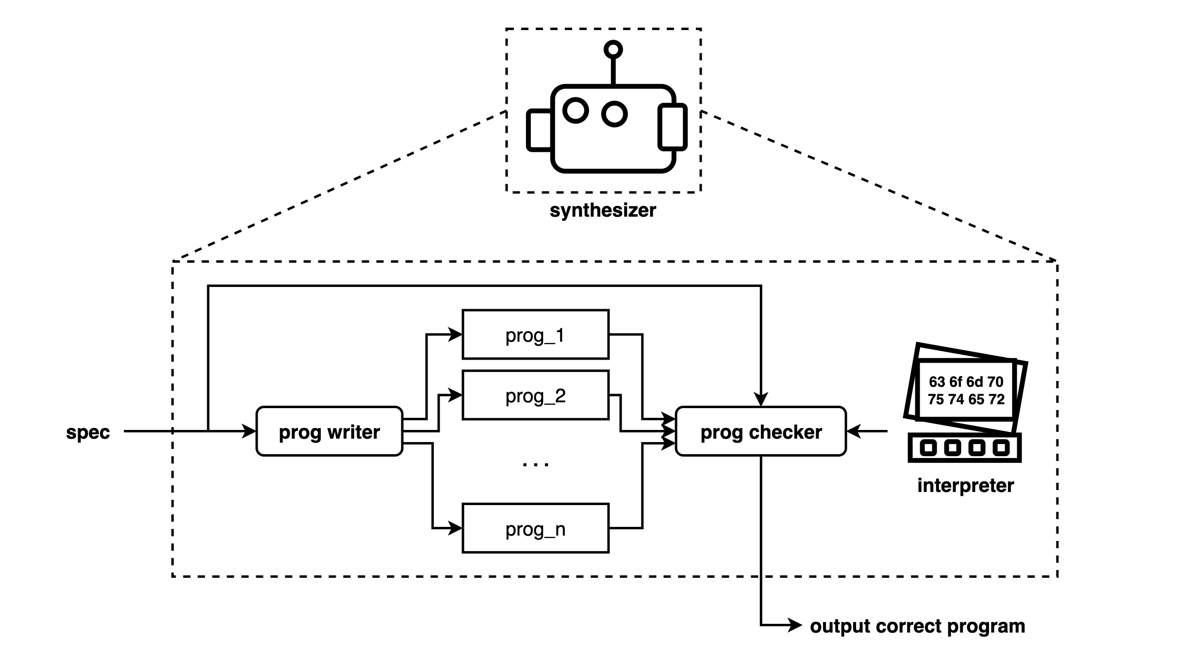
In practice, we resort to rejection sampling from this ground-truth distribution using synthesis.

Given the specification, the program writer proposes (a large number of) programs, then a checker filters the proposals for correctness against the spec.
getting a program-writer close to ground-truth
The “closer” the writer distribution is to the ground-truth, the fewer programs the synthesis algorithm has to sample (i.e. more efficient)2. Closer is formalized as an expected KL-divergence:

Which means, over a prior distribution of specifications P(spec), we want P_writer(prog|spec) be close (small KL divergence) to P_ground-truth(prog|spec).
To obtain program writers that are close to ground-truth, we turn to language models.
language models
A language is a set of strings (a sequence of characters). A language model assigns probabilies over the strings within a language3. Note: the programs in this post are all represented as strings.
unconditional generation
We start with unconditional language models – models that ignore the specifications. Ignoring the specification is certainly a limitation, but it makes a good starting point.

Let’s fix a typical string representing a program, "[1,3,1,4]", as our target to generate. We’ll analyze how well can different unconditional language models generate it.
all strings
We can generate a string by uniformly picking a random character a number of times. This language contains all possible strings of a certain length.
def writer1():
    return ''.join(random.choice(string.printable) for i in range(9))
print(writer1()) # you should see something like "=1Vi![Au37"
A typical program string such as "[1,3,1,4]" has 9 characters, each has a probability of 1 / len(string.printable). Thus this writer has a (1/100)^9 chance of stumbling across it. Not good.
DSL
We can restrict the generation to “strings that look like programs”. This is done with a domain specific language (DSL), which identifies a “reasonable” subset of all-strings as programs. The DSL is specified by a generator – a process capable of generating strings within the DSL4.
def writer2():
    # W is globally defined to be 6
    U = random.randint(0,W)
    D = random.randint(0,W)
    L = random.randint(0,W)
    R = random.randint(0,W)
    return '['+str(U)+','+str(D)+','+str(L)+','+str(R)+']'
print(writer2()) # you should see something like "[5,2,1,0]"
Giving structure to the language, we increased our chance to (1/6)^4 to encounter the program "[1,3,1,4]", despite our DSL containing uninterpretable programs such as "[5,2,1,0]".
better DSL
We can further refine our DSL to be “tighter” to exclude uninterpretable programs.
def writer3():
    U = random.randint(0,W-2)
    L = random.randint(0,W-2)
    height = random.randint(1,W-U)
    width = random.randint(1,W-L)
    D, R = U+height, L+width
    return '['+str(U)+','+str(D)+','+str(L)+','+str(R)+']'
print (writer3()) # you should see something like "[0,2,4,5]"
What’s our chances of stumbling across "[1,3,1,4]" now? I’ll leave the combinatorics to you. Bonus question, is writer3 uniform across all interpretable programs?
synthesis with prior distribution
Unconditional language models gives a prior distribution – how programs are naturally distributed, in the absence of specifications. One can use the prior P(prog) as a writer as-is.

This often resulting in a “good enough” synthesis algorithm for a small space of programs5, and is among the first things a synthesis practictioner will try.
Let’s take a break. no seriously follow along and stretch! the next part will be intense.
training a conditional generator
In conditional generation, a program writer takes spec into account while sampling for plausible programs. We have seen a few from last post. However, it is often simpler to train a parameterized program-writer using data.

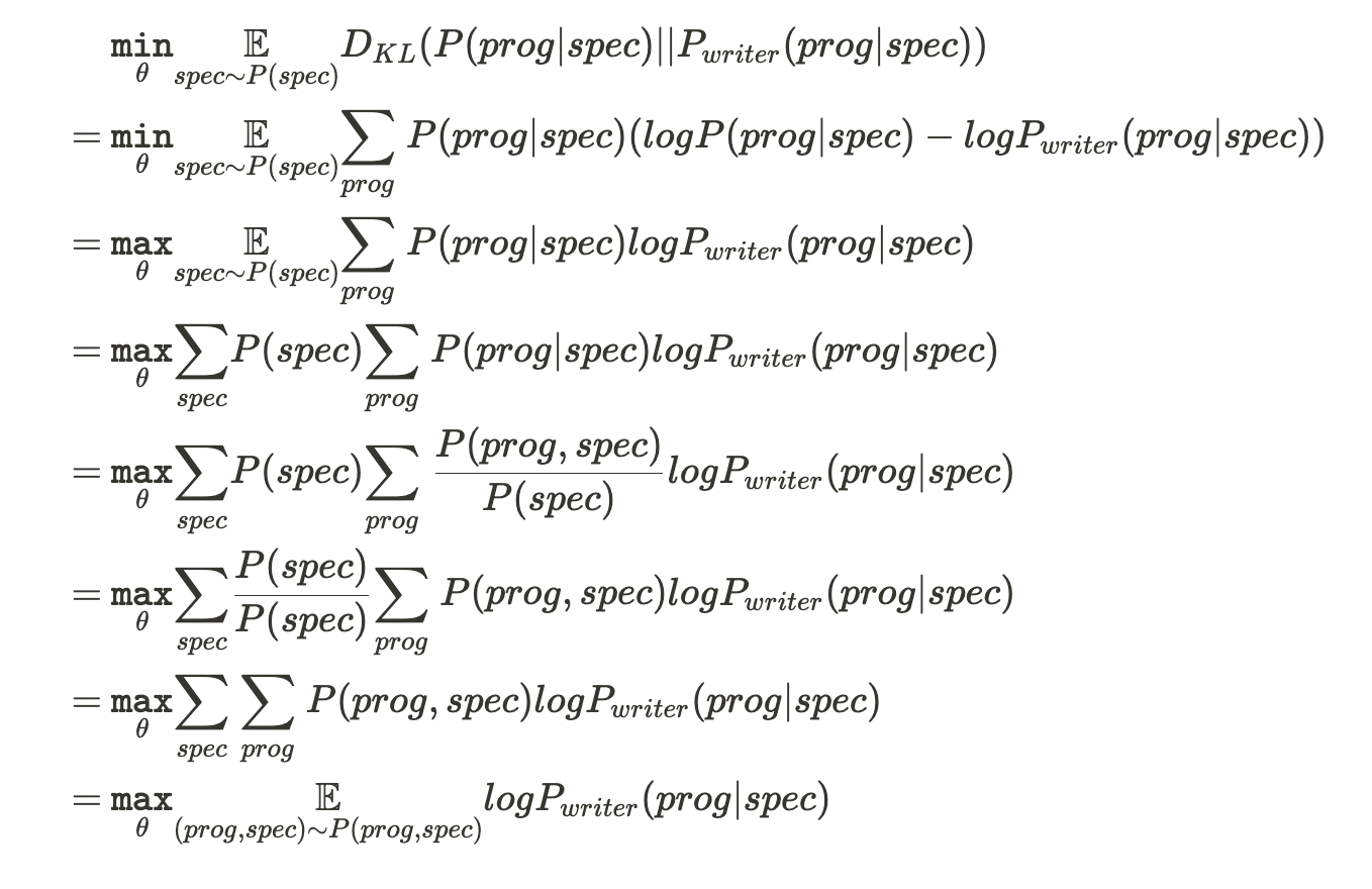
Here, the writer is from a parametric family of functions (e.g. neural networks with weights), and we seek to find a parameter theta that minimizes the expected KL-divergence between our writer distribution and the ground-truth distribution.

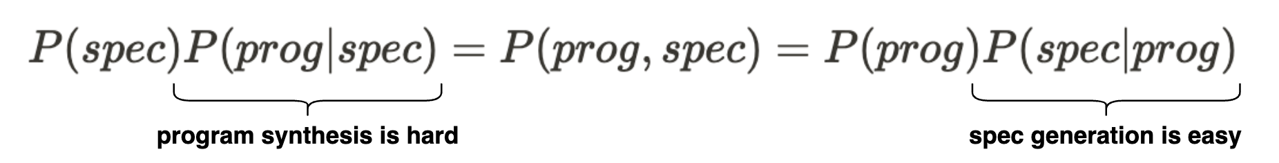
We have a conundrum – To optimize this objective, we need the ground-truth distribution to begin with! We resolve this issue by exploiting the following asymmetry:
the approximation lemma of program synthesis
lemma: Let D be a dataset consisting of (prog,spec) pairs drawn from the joint-distribution P(prog,spec). We can use conditional density estimation on D (i.e. supervised learning) to approximate the ground-truth synthesis distribution 6.
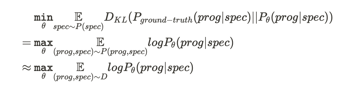
With a big enough dataset D and a flexible enough model class, training the program-writer P_theta(prog|spec) will approach the ground-truth distribution. Moreover, generating D is fully automatic and requires no human annotations! I’ll show you how.
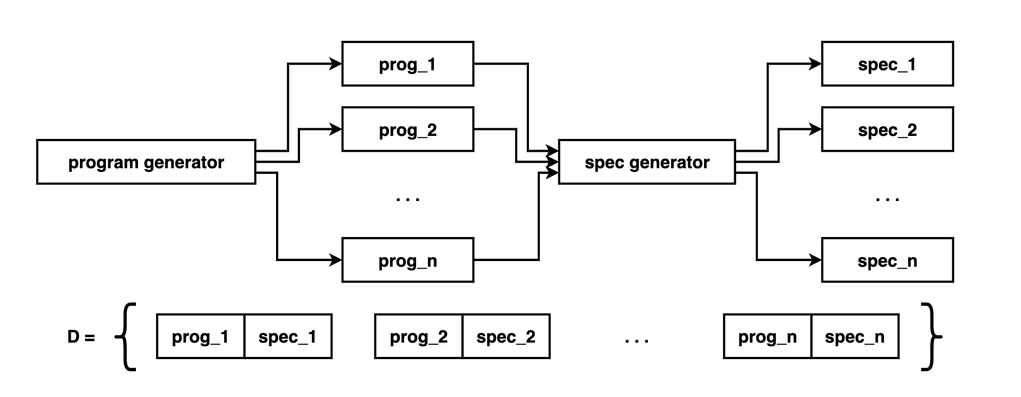
making the dataset D of joint-distribution samples
Each data-point of D is a tuple (prog,spec) from this distribution:

We first generate a program from a prior, then a specification conditioned on this program.
generating programs from a prior
We know how to do this already – this is simply unconditional language generation (e.g. writer3 from earlier). Still, if we can actually obtain a naturalistic dataset of programs, it would serve as a better prior. For instance, codex leveraged the github corpus.
generating specifications from programs
Given a program, we can generate a specification for it by:
- sampling some random inputs
- executing the program to obtain their corresponding outputs.
For our rectangle domain, we first generate some random coordinates (inputs), and see where they lie (outputs) on a given rectangle (program).
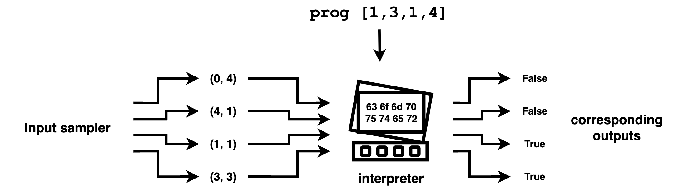
This is what it looks like in code:
def sample_input():
    return random.randint(0,W-1), random.randint(0,W-1)

def sample_spec(prog):
    # pick a number of inputs, up to 10 patches of mushroom / grass total
    n_inputs = random.randint(1,10)
    inputs = [sample_input() for i in range(n_inputs)]
    prog = eval(prog) # needed since for this post progs are modelled as strings
    outputs = [is_inside(prog, input) for input in inputs]
    return list(zip(inputs, outputs))

r_spec = sample_spec("[1,3,1,4]")
print (r_spec) # [((5, 2), False), ((4, 4), False), ((0, 1), False), ((3, 3), True)]
putting it together
This is how you typically generate a dataset D for a given synthesis problem.
def sample_D(n_samples):
D = []
for i in range(n_samples):
prog = writer3()
spec = sample_spec(prog)
D.append((prog, spec))
return D
D = sample_D(10000)
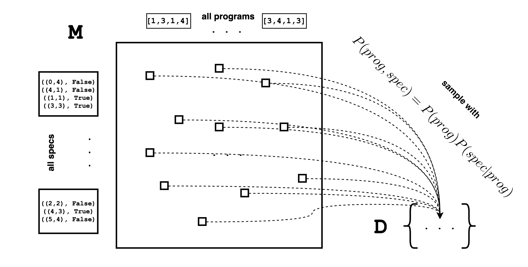
print (D[4542]) # should see something like ('[3,5,4,6]', [((1, 0), False), ((5, 0), False)])D is a sample of M
One should view the dataset D as a sampled summary of the meaning matrix M. While it is impossible to enumerate all entries of M, we can nonetheless take samples from it. By taking more and more samples, we can better observe the landscape of M.
With the dataset D, we’re now ready to do some learning.
phew! let’s take another break. We’re almost done
conditional generation with fitted unigrams
Let’s put the theory into practice using our rectangle example. One of the simplest ways to generate programs is a unigram distribution where, conditioned on the spec, samples each attributes of the program independently. Note that we’re accepting this flawed assumption (the parameters of the rectangles are definitely not independent) for computational simplicity.

We can treat a factor, such as t, as its own multi-way classification problem, mapping the specification to the top boundary (i.e. one of [0, 1, ... W-2]) of the rectangle.
encoding the spec as a vector of binary features
We encode the spec naively as a binary, linearized (WxWx2) feature vector.
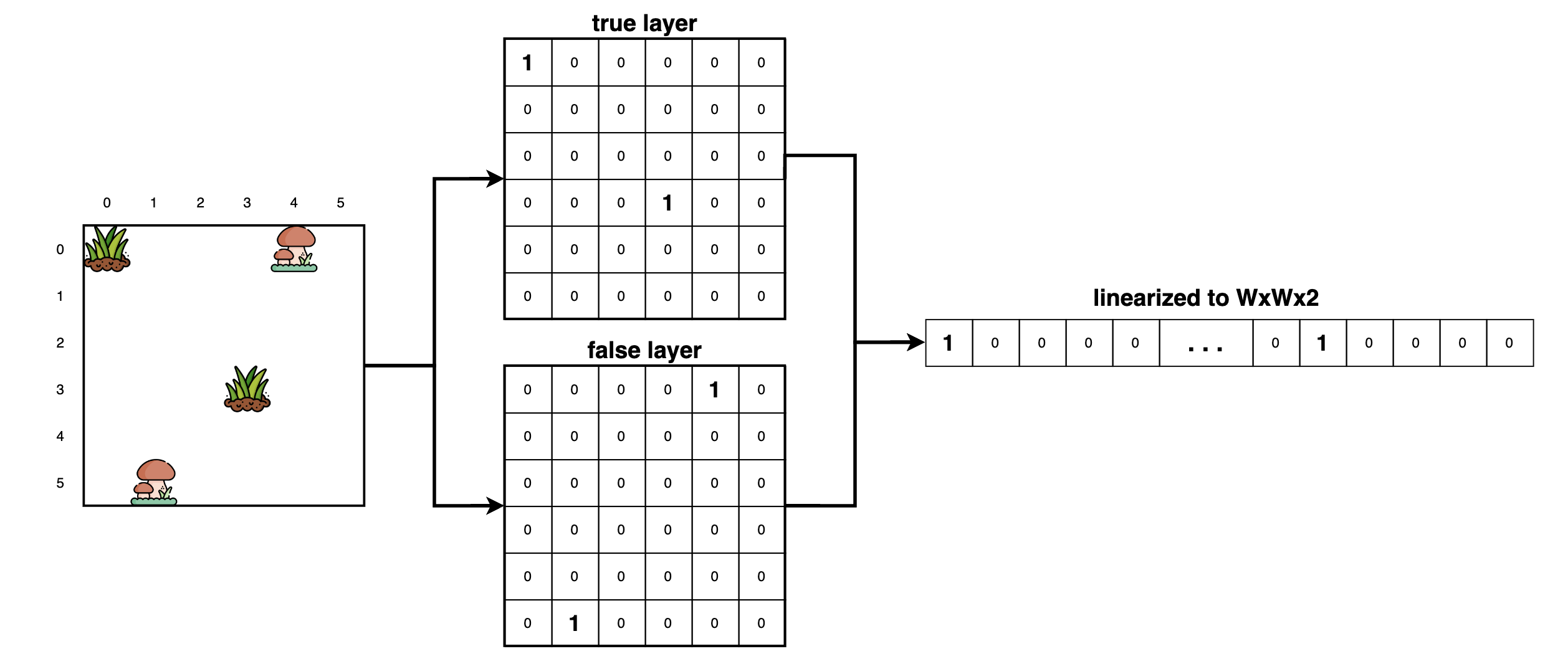
def spec_to_bitvec(spec):
    bitvec = np.zeros((W,W,2))
    for coord,bool in spec:
        # turn bool into a number 0 or 1
        bool_num = 1 if bool else 0
        bitvec[coord[0],coord[1],bool_num] = 1
    # flatten the bitvec into a 1D array
    return bitvec.flatten()
fitting the factors independently
Given our spec feature vector, we fit 4 different conditional unigram distributions, one for each attribute of the rectangle using logisticRegression7. Feel free to experiment with other classifiers such as boosted trees, nearest neighbors, or a conv-net.
import sklearn.linear_model
# train the unigram distribution
def train_unigram(Data):
    spec_bitvec, Ts, Ds, Ls, Rs = [], [], [], [], []
    for prog, spec in Data:
        T, D, L, R = eval(prog)
        spec_bitvec.append(spec_to_bitvec(spec))
        Ts.append(T)
        Ds.append(D)
        Ls.append(L)
        Rs.append(R)
    # convert to numpy arrays
    spec_bitvec = np.array(spec_bitvec)
    Ts = np.array(Ts)
    Ds = np.array(Ds)
    Ls = np.array(Ls)
    Rs = np.array(Rs)
    model_T = sklearn.linear_model.LogisticRegression()
    model_T.fit(spec_bitvec, Ts)
    model_D = sklearn.linear_model.LogisticRegression()
    model_D.fit(spec_bitvec, Ds)
    model_L = sklearn.linear_model.LogisticRegression()
    model_L.fit(spec_bitvec, Ls)
    model_R = sklearn.linear_model.LogisticRegression()
    model_R.fit(spec_bitvec, Rs)
    return model_T, model_D, model_L, model_R
making a program-writer using the fitted unigrams
Once our conditional unigram distribution is fitted, we can use it to write programs at inference time. Each attribute of the rectangle will be sampled independently, and put together to form a (hopefully valid) rectangle.
def get_writer4(model_T, model_D, model_L, model_R):
    def writer4(spec):
        spec_bitvec = spec_to_bitvec(spec)
        model_T_prob = model_T.predict_proba([spec_bitvec])[0]
        model_T_sample = np.random.choice(range(len(model_T_prob)), p=model_T_prob)
        model_D_prob = model_D.predict_proba([spec_bitvec])[0]
        model_D_sample = np.random.choice(range(len(model_D_prob)), p=model_D_prob)
        model_L_prob = model_L.predict_proba([spec_bitvec])[0]
        model_L_sample = np.random.choice(range(len(model_L_prob)), p=model_L_prob)
        model_R_prob = model_R.predict_proba([spec_bitvec])[0]
        model_R_sample = np.random.choice(range(len(model_R_prob)), p=model_R_prob)
        return '[{},{},{},{}]'.format(model_T_sample, model_D_sample, model_L_sample, model_R_sample)
    return writer4
compare different language models as program writers
We can now create different program synthesizers by using different conditional and un-conditional writers, including the manual better_writer algorithm from last post:
# ignoring the spec for unconditional writers
synthesizer1 = get_synthesizer(lambda spec : writer1(), is_correct, 100)
synthesizer2 = get_synthesizer(lambda spec : writer2(), is_correct, 100)
synthesizer3 = get_synthesizer(lambda spec : writer3(), is_correct, 100)
# our fitted unigram writer
synthesizer4 = get_synthesizer(get_writer4(*train_unigram(D_train)), is_correct, 100)
# the manual writer from last post
synthesizer5 = get_synthesizer(manual_writer, is_correct, 100)
The customary plot comparing different synthesis algorithms shows search budget on the x axis, and fraction of tasks solved on the y axis. To generate this plot, we make a test set D_test and run all our contestant synthesizers on it, keeping track of how many samples each synthesizer required before a solution is found.
    to_plot = [[], [], [], [], []]
    for _, spec in D_test:
        for synth_id, synth in enumerate([synthesizer1, synthesizer2, synthesizer3, synthesizer4, synthesizer5]):
            samples_needed, prog = synth(spec)
            to_plot[synth_id].append(samples_needed)
    print (to_plot)
We then iterate over different budgets, from 0 to 100, and count how many synthesis tasks can be solved with equal or less budget. Do this for each of the synthesizers produces the following plot:
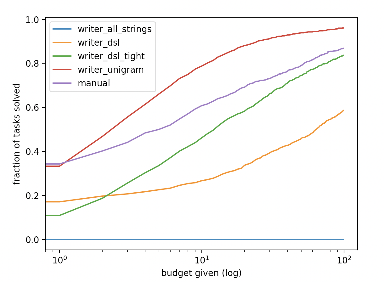
As we can see, our fitted unigram writer performs even better than the manual solution.
code
All code for this post can be found here. It depends on rectangle.py
exercise
Extend the unigram generation above to bigram generation8 instead, does it perform better?
conclusion
In this post we covered how to obtain several reasonable program writers, including the generating from the prior, and by training on synthetically generated data.
– evan 2022-08-29
up next
The next post cover we’ll cover how to fine-tune a large language model for the same task, which offers additional flexibilities. let’s go for it
notes
-
This is not entirely accurate. In practice, we’re often interested in finding just one correct program instead of uniformly sampling from every correct program. ↩
-
You can find good resources online about language modeling, such as CS324 - intro to large language models from Stanford or a video on language modeling by Karpathy. ↩
-
On one hand, any data structure (think json) that can be “executed” on an interpreter you’ve build is a DSL. On the other hand, you can get fairly deep into building a compiler (see you in a year!). I’d start with something simple like this or this. ↩
-
Enumerative synthesis such as lambda-squared by John Feser uses program-length prior distribution (longer programs are less likely) and aggressive space-pruning. ↩
-
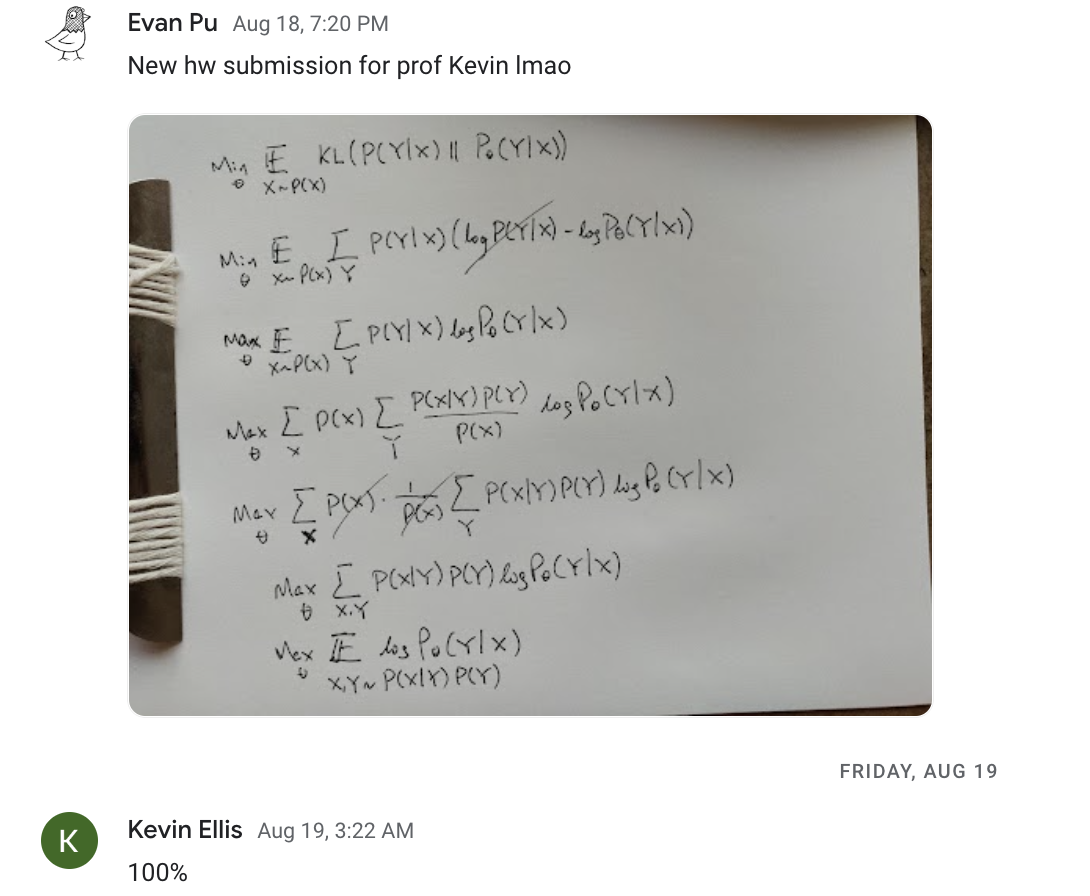
Full derivation typical in the style of variational inference with kevin’s approval. ↩
-
Kevin Ellis leverages bigram enumeration for his dream-coder system ↩